https://www.dsprelated.com/freeb ... alysis_Windows.html
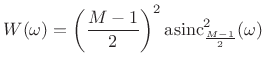
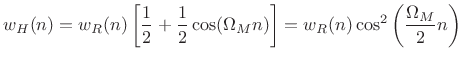
In spectrum analysis of naturally occurring audio signals, we nearly always analyze a short segment of a signal, rather than the whole signal. This is the case for a variety of reasons. Perhaps most fundamentally, the ear similarly Fourier analyzes only a short segment of audio signals at a time (on the order of 10-20 ms worth). Therefore, to perform a spectrum analysis having time- and frequency-resolution comparable to human hearing, we must limit the time-window accordingly. We will see that the proper way to extract a ``short time segment'' of length  from a longer signal is to multiply it by a window function such as the Hann window: from a longer signal is to multiply it by a window function such as the Hann window:
We will see that the main benefit of choosing a good Fourier analysis window function is minimization of side lobes, which cause ``cross-talk'' in the estimated spectrum from one frequency to another. The study of spectrum-analysis windows serves other purposes as well. Most immediately, it provides an array of useful window types which are best for different situations. Second, by studying windows and their Fourier transforms, we build up our knowledge of Fourier dualities in general. Finally, the defining criteria for different window types often involve interesting and useful analytical techniques. In this chapter, we begin with a summary of the rectangular window, followed by a variety of additional window types, including the generalized Hamming and Blackman-Harris families (sums of cosines), Bartlett (triangular), Poisson (exponential), Kaiser (Bessel), Dolph-Chebyshev, Gaussian, and other window types.
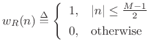
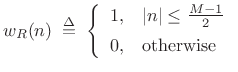
THE RECTANGULAR WINDOWThe (zero-centered) rectangular window may be defined by
where  is the window length in samples (assumed odd for now). A plot of the rectangular window appears in Fig.3.1 for length is the window length in samples (assumed odd for now). A plot of the rectangular window appears in Fig.3.1 for length  . It is sometimes convenient to define windows so that their dc gain is 1, in which case we would multiply the definition above by . It is sometimes convenient to define windows so that their dc gain is 1, in which case we would multiply the definition above by  . .
Figure 3.1: The rectangular window.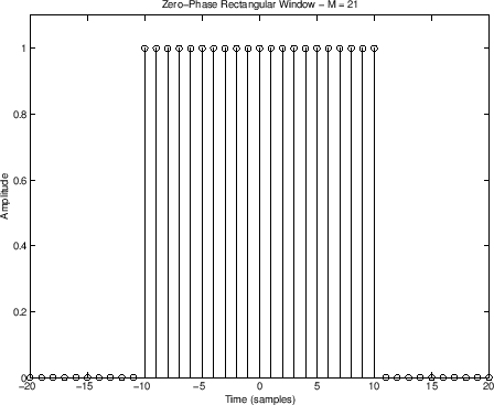
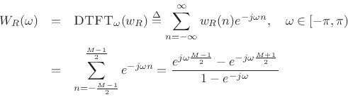
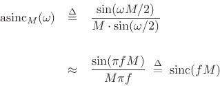
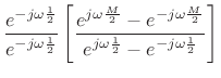
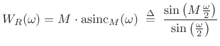
We can factor out linear phase terms from the numerator and denominator of the above expression to get
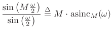
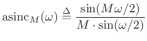
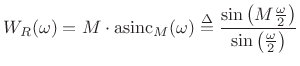
where  denotes the aliased sinc function:4.1 denotes the aliased sinc function:4.1
(also called the Dirichlet function [175,72] or periodic sinc function). This (real) result is for thezero-centered rectangular window. For the causal case, a linear phase term appears:
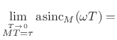
The term ``aliased sinc function'' refers to the fact that it may be simply obtained by samplingthe length- continuous-time rectangular window, which has Fourier transform sinc continuous-time rectangular window, which has Fourier transform sinc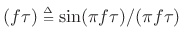 (given amplitude (given amplitude  in the time domain). Sampling at intervals of in the time domain). Sampling at intervals of  seconds in the time domain corresponds to aliasing in the frequency domain over the interval seconds in the time domain corresponds to aliasing in the frequency domain over the interval  Hz, and by direct derivation, we have found the result. It is interesting to consider what happens as the window duration increases continuously in the time domain: the magnitude spectrum can only change in discrete jumps as new samples are included, even though it is continuously parametrized in . Hz, and by direct derivation, we have found the result. It is interesting to consider what happens as the window duration increases continuously in the time domain: the magnitude spectrum can only change in discrete jumps as new samples are included, even though it is continuously parametrized in . As the sampling rate goes to infinity, the aliased sinc function therefore approaches the sinc function
sinc 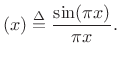 | (4.7) |
Specifically,
 sinc  | (4.8) |
where  .4.2 .4.2
Figure 3.2: Fourier transform of the rectangular window.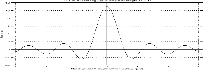
Figure 3.2 illustrates 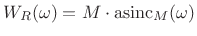 for for  . Note that this is the complete window transform, not just its real part. We obtain real window transforms like this only for zero-centered, symmetric windows. Note that the phase of rectangular-window transform . Note that this is the complete window transform, not just its real part. We obtain real window transforms like this only for zero-centered, symmetric windows. Note that the phase of rectangular-window transform  is zero for is zero for  , which is the width of the main lobe. This is why zero-centered windows are often called zero-phase windows; while the phase actually alternates between 0 and , which is the width of the main lobe. This is why zero-centered windows are often called zero-phase windows; while the phase actually alternates between 0 and  radians, the values occur only within side-lobes which are routinely neglected (in fact, the window is normally designed to ensure that all side-lobes can be neglected). radians, the values occur only within side-lobes which are routinely neglected (in fact, the window is normally designed to ensure that all side-lobes can be neglected). More generally, we may plot both the magnitude and phase of the window versus frequency, as shown in Figures 3.4 and 3.5 below. In audio work, we more typically plot the window transform magnitude on a decibel (dB) scale, as shown in Fig.3.3 below. It is common to normalize the peak of the dB magnitude to 0 dB, as we have done here.
Figure 3.3: Magnitude (dB) of the rectangular-window transform.
Figure 3.4: Magnitude of the rectangular-window Fourier transform.
Figure 3.5: Phase of the rectangular-window Fourier transform.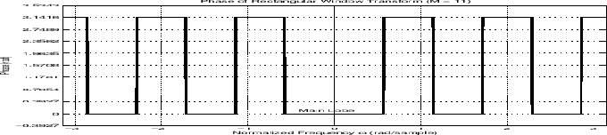
RECTANGULAR WINDOW SIDE-LOBESFrom Fig.3.3 and Eq. (3.4), we see that the main-lobe width is (3.4), we see that the main-lobe width is  radian, and the side-lobe level is 13 dB down. radian, and the side-lobe level is 13 dB down.
Figure 3.6: Roll-off of the rectangular-window Fourier transform.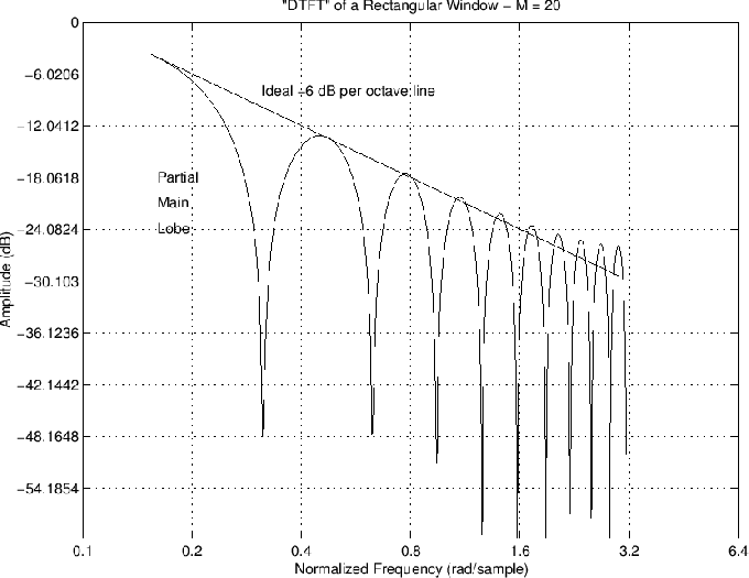
As the sampling rate approaches infinity, the rectangular window transform (  ) converges exactly to the sinc function. Therefore, the departure of the roll-off from that of the sinc function can be ascribed to aliasing in the frequency domain, due to sampling in the time domain (hence the name `` ''). ) converges exactly to the sinc function. Therefore, the departure of the roll-off from that of the sinc function can be ascribed to aliasing in the frequency domain, due to sampling in the time domain (hence the name `` ''). Note that each side lobe has width 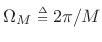 , as measured between zero crossings.4.3The main lobe, on the other hand, is width , as measured between zero crossings.4.3The main lobe, on the other hand, is width  . Thus, in principle, we should never confuse side-lobe peaks with main-lobe peaks, because a peak must be at least wide in order to be considered ``real''. However, in complicated real-world scenarios, side-lobes can still cause estimation errors (``bias''). Furthermore, two sinusoids at closely spaced frequencies and opposite phase can partially cancel each other's main lobes, making them appear to be narrower than . . Thus, in principle, we should never confuse side-lobe peaks with main-lobe peaks, because a peak must be at least wide in order to be considered ``real''. However, in complicated real-world scenarios, side-lobes can still cause estimation errors (``bias''). Furthermore, two sinusoids at closely spaced frequencies and opposite phase can partially cancel each other's main lobes, making them appear to be narrower than .
Thus, it has zero crossings at integer multiples of
Its main-lobe width is and its first side-lobe is 13 dB down from the main-lobe peak. As gets bigger, the main-lobe narrows, giving better frequency resolution (as discussed in the next section). Note that the window-length has no effect on side-lobe level (ignoring aliasing). The side-lobe height is instead a result of the abruptness of the window's transition from 1 to 0 in the time domain. This is the same thing as the so-called Gibbs phenomenonseen in truncated Fourier series expansions of periodic waveforms. The abruptness of the window discontinuity in the time domain is also what determines the side-lobe roll-off rate (approximately 6 dB per octave). The relation of roll-off rate to the smoothness of the window at its endpoints is discussed in §B.18.
RECTANGULAR WINDOW SUMMARYThe rectangular window was discussed in Chapter 5 (§3.1). Here we summarize the results of that discussion.
Definition ( odd):
Transform:
The DTFT of a rectangular window is shown in Fig.3.7.
Figure 3.7: Rectangular window discrete-time Fourier transform.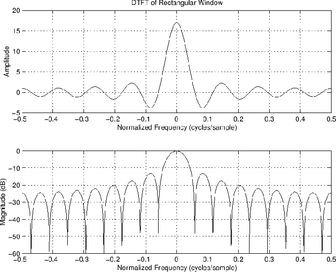
Properties: - Zero crossings at integer multiples of
- Main lobe width is
 . . - As increases, the main lobe narrows (better frequency resolution).
- has no effect on the height of the side lobes (same as the ``Gibbs phenomenon'' for truncated Fourier series expansions).
- First side lobe only 13 dB down from the main-lobe peak.
- Side lobes roll off at approximately 6dB per octave.
- A phase term arises when we shift the window to make it causal, while the window transform is real in the zero-phase case (i.e., centered about time 0).
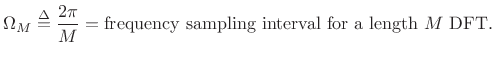
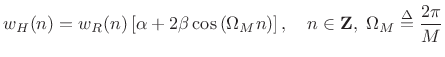
GENERALIZED HAMMING WINDOW FAMILYThe generalized Hamming window family is constructed by multiplying a rectangular window by one period of a cosine. The benefit of the cosine tapering is lower side-lobes. The price for this benefit is that the main-lobe doubles in width. Two well known members of the generalized Hamming family are the Hann and Hamming windows, defined below. The basic idea of the generalized Hamming family can be seen in the frequency-domainpicture of Fig.3.8. The center dotted waveform is the aliased sinc function 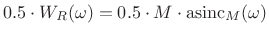 (scaled rectangular window transform). The other two dotted waveforms are scaled shifts of the same function, (scaled rectangular window transform). The other two dotted waveforms are scaled shifts of the same function, 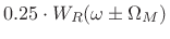 . The sum of all three dotted waveforms gives the solid line. We see that . The sum of all three dotted waveforms gives the solid line. We see that - there is some cancellation of the side lobes, and
- the width of the main lobe is doubled.
Figure 3.8: Construction of the generalized Hamming window transform as a superposition of three shifted aliased sinc functions.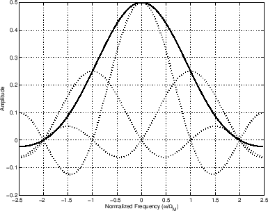
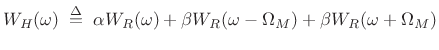
In terms of the rectangular window transform (the zero-phase, unit-amplitude case), this can be written as
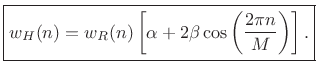
where  , ,  in the example of Fig.3.8. in the example of Fig.3.8.Using the shift theorem (§2.3.4), we can take the inverse transform of the above equation to obtain
or,
Choosing various parameters for  and and  result in different windows in the generalized Hamming family, some of which have names. result in different windows in the generalized Hamming family, some of which have names.
HANN OR HANNING OR RAISED COSINEThe Hann window (or hanning or raised-cosine window) is defined based on the settings and in (3.17):
where .The Hann window and its transform appear in Fig.3.9. The Hann window can be seen as one period of a cosine ``raised'' so that its negative peaks just touch zero (hence the alternate name ``raised cosine''). Since it reaches zero at its endpoints with zero slope, the discontinuity leaving the window is in the second derivative, or the third term of its Taylor series expansion at an endpoint. As a result, the side lobes roll off approximately 18 dB per octave. In addition to the greatly accelerated roll-off rate, the first side lobe has dropped from  dB (rectangular-window case) down to dB (rectangular-window case) down to  dB. The main-lobe width is of course double that of the rectangular window. For Fig.3.9, the window was computed in Matlab as hanning(21). Therefore, it is the variant that places the zero endpoints one-half sample to the left and right of the outermost window samples (see next section). dB. The main-lobe width is of course double that of the rectangular window. For Fig.3.9, the window was computed in Matlab as hanning(21). Therefore, it is the variant that places the zero endpoints one-half sample to the left and right of the outermost window samples (see next section).
Figure 3.9: The Hann window (hanning(21)) and its DTFT.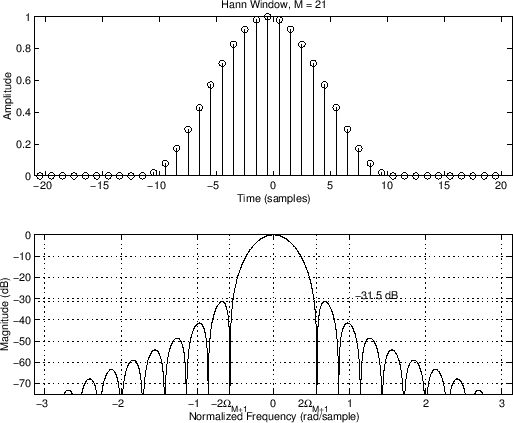
MATLAB FOR THE HANN WINDOWw = hanning(M);which, in Matlab only is equivalent tow = .5*(1 - cos(2*pi*(1:M)'/(M+1)));For  , hanning(3) returns the following:>> hanning(3)ans = 0.5 1 0.5Note the curious use of M+1 in the denominator instead of M as we would expect from the family definition in (3.17). This perturbation serves to avoid using zero samples in the window itself. (Why bother to multiply explicitly by zero?) Thus, the Hann window as returned by Matlab hanning function reaches zero one sample beyond the endpoints to the left and right. The minus sign, which differs from (3.18), serves to make the window causal instead of zero phase.>> hann(3)ans = 0 1 0This case is equivalent to the following matlab expression:w = .5*(1 - cos(2*pi*(0:M-1)'/(M-1)));The use of , hanning(3) returns the following:>> hanning(3)ans = 0.5 1 0.5Note the curious use of M+1 in the denominator instead of M as we would expect from the family definition in (3.17). This perturbation serves to avoid using zero samples in the window itself. (Why bother to multiply explicitly by zero?) Thus, the Hann window as returned by Matlab hanning function reaches zero one sample beyond the endpoints to the left and right. The minus sign, which differs from (3.18), serves to make the window causal instead of zero phase.>> hann(3)ans = 0 1 0This case is equivalent to the following matlab expression:w = .5*(1 - cos(2*pi*(0:M-1)'/(M-1)));The use of  is necessary to include zeros at both endpoints. The Matlab hann function is a special case of what Matlab calls ``generalized cosine windows'' (type gencoswin). is necessary to include zeros at both endpoints. The Matlab hann function is a special case of what Matlab calls ``generalized cosine windows'' (type gencoswin).In Matlab, both hann(3,'periodic') and hanning(3,'periodic') produce the following window: >> hann(3,'periodic')ans = 0 0.75 0.75This case is equivalent tow = .5*(1 - cos(2*pi*(0:M-1)'/M));which agrees (finally) with definition (3.18). We see that in this case, the left zero endpoint is included in the window, while the one on the right lies one sample outside to the right. In general, the 'periodic' window option asks for a window that can be overlapped and added to itself at certain time displacements ( samples in this case) to produce a constant function. Use of ``periodic'' windows in this way is introduced in §7.3 and discussed more fully in Chapters [url=https://www.dsprelated.com/freebooks/sasp/Overlap_Add_OLA_STFT_Processing.html#chap samples in this case) to produce a constant function. Use of ``periodic'' windows in this way is introduced in §7.3 and discussed more fully in Chapters [url=https://www.dsprelated.com/freebooks/sasp/Overlap_Add_OLA_STFT_Processing.html#chap la]8[/url] and 9. la]8[/url] and 9.In Octave, both the hann and hanning functions include the endpoint zeros. In practical applications, it is safest to write your own window functions in the matlab language in order to ensure portability and consistency. After all, they are typically only one line of code! In comparing window properties below, we will speak of the Hann window as having a main-lobe width equal to  , and a side-lobe width , and a side-lobe width  , even though in practice they may really be , even though in practice they may really be  and and  , respectively, as illustrated above. These remarks apply to all windows in the generalized Hamming family, as well as the Blackman-Harris family introduced in §3.3below. , respectively, as illustrated above. These remarks apply to all windows in the generalized Hamming family, as well as the Blackman-Harris family introduced in §3.3below.
Summary of Hann window properties: - Main lobe is wide,
- First side lobe at -31dB
- Side lobes roll off approximately
 dB per octave dB per octave
HAMMING WINDOWThe Hamming window is determined by choosing in (3.17) (with  ) to cancel the largest side lobe [101].4.4 Doing this results in the values ) to cancel the largest side lobe [101].4.4 Doing this results in the values
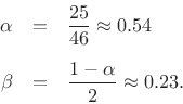
The peak side-lobe level is approximately  dB for the Hamming window [101].4.5 It happens that this choice is very close to that which minimizes peak side-lobe level (down to dB for the Hamming window [101].4.5 It happens that this choice is very close to that which minimizes peak side-lobe level (down to  dB--the lowest possible within the generalized Hamming family) [196]: dB--the lowest possible within the generalized Hamming family) [196]:
Since rounding the optimal to two significant digits gives  , the Hamming window can be considered the ``Chebyshev Generalized Hamming Window'' (approximately). Chebyshev-type designs normally exhibit equiripple error behavior, because the worst-case error (side-lobe level in this case) is minimized. However, within the generalized Hamming family, the asymptotic spectral roll-off is constrained to be at least , the Hamming window can be considered the ``Chebyshev Generalized Hamming Window'' (approximately). Chebyshev-type designs normally exhibit equiripple error behavior, because the worst-case error (side-lobe level in this case) is minimized. However, within the generalized Hamming family, the asymptotic spectral roll-off is constrained to be at least  dB per octave due to the form (3.17) of all windows in the family. We'll discuss the true Chebyshev window in §3.10 below; we'll see that it is not monotonic from its midpoint to an endpoint, and that it is in fact impulsive at its endpoints. (To peek ahead at a Chebyshev window and transform, see Fig.3.31.) Generalized Hamming windows can have a step discontinuity at their endpoints, but no impulsive points. dB per octave due to the form (3.17) of all windows in the family. We'll discuss the true Chebyshev window in §3.10 below; we'll see that it is not monotonic from its midpoint to an endpoint, and that it is in fact impulsive at its endpoints. (To peek ahead at a Chebyshev window and transform, see Fig.3.31.) Generalized Hamming windows can have a step discontinuity at their endpoints, but no impulsive points.
Figure 3.10: A Hamming window and its transform.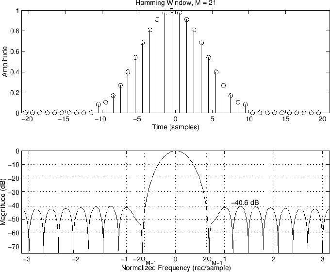
The Hamming window and its DTFT magnitude are shown in Fig.3.10. Like the Hann window, the Hamming window is also one period of a raised cosine. However, the cosine is raised so high that its negative peaks are above zero, and the window has a discontinuity in amplitudeat its endpoints (stepping discontinuously from 0.08 to 0). This makes the side-lobe roll-off rate very slow (asymptotically dB/octave). On the other hand, the worst-case side lobe plummets to  dB,4.6which is the purpose of the Hamming window. This is 10 dB better than the Hann case of Fig.3.9 and 28 dB better than the rectangular window. The main lobe is approximately wide, as is the case for all members of the generalized Hamming family ( dB,4.6which is the purpose of the Hamming window. This is 10 dB better than the Hann case of Fig.3.9 and 28 dB better than the rectangular window. The main lobe is approximately wide, as is the case for all members of the generalized Hamming family (  ). ). Due to the step discontinuity at the window boundaries, we expect a spectral envelope which is an aliased version of a dB per octave (i.e., a  roll-off is converted to a ``cosecant roll-off'' by aliasing, as derived in §3.1 and illustrated in Fig.3.6). However, for the Hamming window, the side-lobes nearest the main lobe have been strongly shaped by the optimization. As a result, the nearly dB per octave roll-off occurs only over an interior interval of the spectrum, well between the main lobe and half the sampling rate. This is easier to see for a larger , as shown in Fig.3.11, since then the optimized side-lobes nearest the main lobe occupy a smaller frequency interval about the main lobe. roll-off is converted to a ``cosecant roll-off'' by aliasing, as derived in §3.1 and illustrated in Fig.3.6). However, for the Hamming window, the side-lobes nearest the main lobe have been strongly shaped by the optimization. As a result, the nearly dB per octave roll-off occurs only over an interior interval of the spectrum, well between the main lobe and half the sampling rate. This is easier to see for a larger , as shown in Fig.3.11, since then the optimized side-lobes nearest the main lobe occupy a smaller frequency interval about the main lobe.
Figure 3.11: A longer Hamming window and its transform.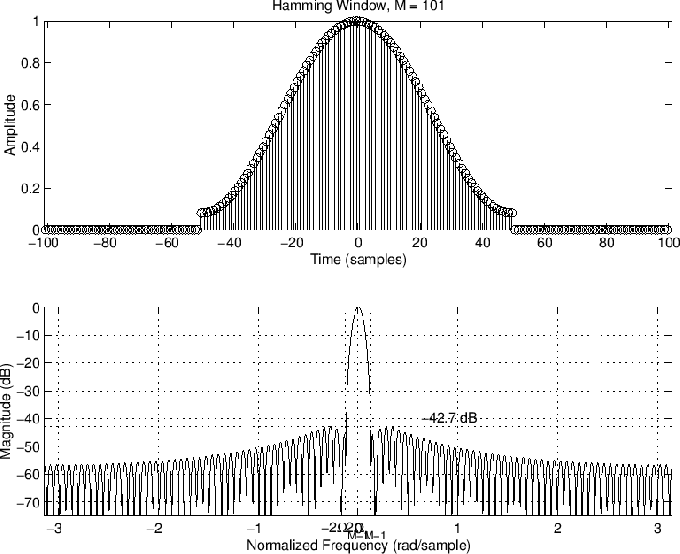
Since the Hamming window side-lobe level is more than 40 dB down, it is often a good choice for ``1% accurate systems,'' such as 8-bit audio signal processing systems. This is because there is rarely any reason to require the window side lobes to lie far below the signal quantization noise floor. The Hamming window has been extensively used in telephone communications signal processing wherein 8-bit CODECs were standard for many decades (albeit  -law encoded). For higher quality audio signal processing, higher quality windows may be required, particularly when those windows act as lowpass filters (as developed in Chapter 9). -law encoded). For higher quality audio signal processing, higher quality windows may be required, particularly when those windows act as lowpass filters (as developed in Chapter 9).
MATLAB FOR THE HAMMING WINDOWw = hamming(M);which is equivalent tow = .54 - .46*cos(2*pi*(0:M-1)'/(M-1));Note that M-1 is used in the denominator rather than M+1 as in the Hann window case. Since the Hamming window cannot reach zero for any choice of samples of the defining raised cosine, it makes sense not to have M+1 here. Using M-1 (instead of M) provides that the returned window is symmetric, which is usually desired. However, we will learn later that there are times when M is really needed in the denominator (such as when the window is being used successively over time in an overlap-add scheme, in which case the sum of overlapping windows must be constant).The hamming function in the Matlab Signal Processing Tool Box has an optional argument 'periodic' which effectively uses instead of . The default case is 'symmetric'. The following examples should help clarify the difference: >> hamming(3) % same in Matlab and Octaveans = 0.0800 1.0000 0.0800>> hamming(3,'symmetric') % Matlab onlyans = 0.0800 1.0000 0.0800>> hamming(3,'periodic') % Matlab onlyans = 0.0800 0.7700 0.7700>> hamming(4) % same in Matlab and Octaveans = 0.0800 0.7700 0.7700 0.0800
SUMMARY OF GENERALIZED HAMMING WINDOWS
Definition:
where
Transform:
where
Common Properties - Rectangular + scaled-cosine window
- Cosine has one period across the window
- Symmetric (
 zero or linear phase) zero or linear phase) - Positive (by convention on and )
- Main lobe is radians per sample wide, where
 - Zero-crossings (``notches'') in window transform at intervals of outside of main lobe
Figure 3.12 compares the window transforms for the rectangular, Hann, and Hamming windows. Note how the Hann window has the fastest roll-off while the Hamming window is closest to being equal-ripple. The rectangular window has the narrowest main lobe.
Figure 3.12: Comparison of window transforms for the rectangular, Hann, and Hamming windows.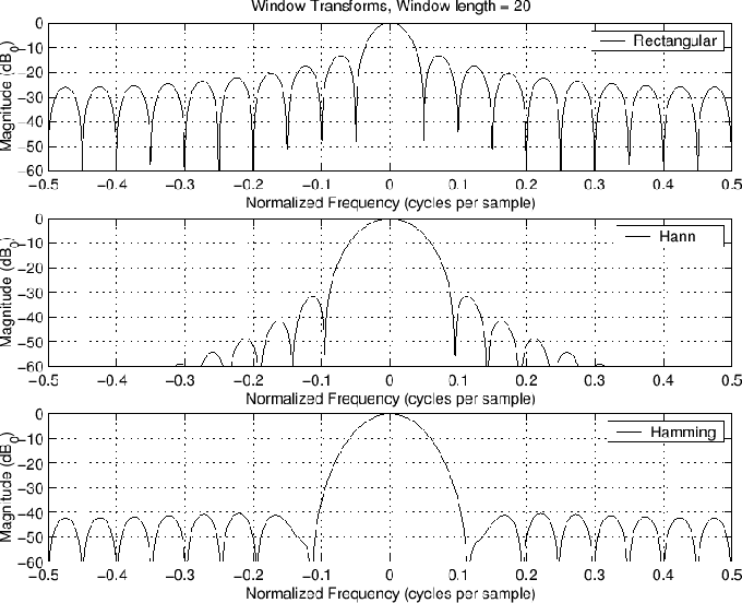
Rectangular window properties: - Abrupt transition from 1 to 0 at the window endpoints
- Roll-off is asymptotically dB per octave (as
 ) ) - First side lobe is dB relative to main-lobe peak
Hann window properties: - Smooth transition to zero at window endpoints
- Roll-off is asymptotically -18 dB per octave
- First side lobe is
 dB relative to main-lobe peak dB relative to main-lobe peak
Hamming window properties: - Discontinuous ``slam to zero'' at endpoints
- Roll-off is asymptotically -6 dB per octave
- Side lobes are closer to ``equal ripple''
- First side lobe is
 dB down = dB down =  dB better than Hann4.7 dB better than Hann4.7
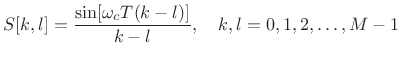
THE MLT SINE WINDOWThe modulated lapped transform (MLT) [160] uses the sine window, defined by
The sine window is used in MPEG-1, Layer 3 (MP3 format), MPEG-2 AAC, and MPEG-4 [200].
Properties: Note that in perceptual audio coding systems, there is both an analysis window and a synthesis window. That is, the sine window is deployed twice, first when encoding the signal, and second when decoding. As a result, the sine window is squared in practical usage, rendering it equivalent to a Hann window ( ) in the final output signal (when there are no spectral modifications). ) in the final output signal (when there are no spectral modifications). It is of great practical value that the second window application occurs after spectral modifications (such as spectral quantization); any distortions due to spectral modifications are tapered gracefully to zero by the synthesis window. Synthesis windows were introduced at least as early as 1980 [213,49], and they became practical for audio coding with the advent of time-domain aliasing cancellation (TDAC) [214]. The TDAC technique made it possible to use windows with 50% overlap without suffering a doubling of the number of samples in the short-time Fourier transform. TDAC was generalized to ``lapped orthogonal transforms'' (LOT) by Malvar [160]. The modulated lapped transform (MLT) is a variant of LOT used in conjunction with the modulated discrete cosine transform (MDCT) [160]. See also [287] and [291].
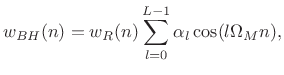
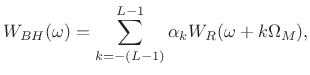
BLACKMAN-HARRIS WINDOW FAMILYThe Blackman-Harris (BH) window family is a straightforward generalization of the Hamming family introduced in §3.2. Recall from that discussion that the generalized Hamming family was constructed using a summation of three shifted and scaled aliased-sinc-functions(shown in Fig.3.8). The Blackman-Harris family is obtained by adding still more shifted sinc functions:
where , and  is the length zero-phase rectangular window (nonzero for is the length zero-phase rectangular window (nonzero for 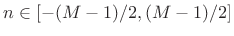 ). The corresponding window transform is given by ). The corresponding window transform is given by
where denotes the rectangular-window transform, and  as usual. as usual.Note that for  , we obtain the rectangular window, and for , we obtain the rectangular window, and for  , the BH family specializes to the generalized Hamming family. , the BH family specializes to the generalized Hamming family.
BLACKMAN WINDOW FAMILY
Relative to the generalized Hamming family (§3.2), we have added one more cosine weighted by  . We now therefore have three degrees of freedom to work with instead of two. In the Hamming family, we used one degree of freedom to normalize the window amplitude and the second was used either to maximize roll-off rate (Hann) or side-lobe rejection (Hamming). Now we can use two remaining degrees of freedom (after normalization) to optimize these objectives, or we can use one for each, resulting in three subtypes within the Blackman window family. . We now therefore have three degrees of freedom to work with instead of two. In the Hamming family, we used one degree of freedom to normalize the window amplitude and the second was used either to maximize roll-off rate (Hann) or side-lobe rejection (Hamming). Now we can use two remaining degrees of freedom (after normalization) to optimize these objectives, or we can use one for each, resulting in three subtypes within the Blackman window family.
CLASSIC BLACKMANThe so-called ``Blackman Window'' is the specific case for which   , and , and  . It has the following properties: . It has the following properties: - Side lobes roll off at about
 per octave (like Hann) per octave (like Hann) - Side-lobe level is about
 dB (worst case) dB (worst case) - One degree of freedom used to increase the roll-off rate from 6dB/octave (like rectangular) to 18 dB per octave by matching amplitude and slope to 0 at the window endpoints
- One degree of freedom is used to minimize side lobes (like Hamming)
- One degree of freedom is used to scale the window
MATLAB FOR THE CLASSIC BLACKMAN WINDOW
N = 101; L = 3; No2 = (N-1)/2; n=-No2:No2;ws = zeros(L,3*N); z = zeros(1,N);for l=0 -1 ws(l+1, -1 ws(l+1, = [z,cos(l*2*pi*n/N),z];endalpha = [0.42,0.5,0.08]; % Classic Blackmanw = alpha * ws; = [z,cos(l*2*pi*n/N),z];endalpha = [0.42,0.5,0.08]; % Classic Blackmanw = alpha * ws;
Figure 3.13: Classic Blackman window and transform.
THREE-TERM BLACKMAN-HARRIS WINDOWThe classic Blackman window of the previous section is a three-term window in the Blackman-Harris family ( ), in which one degree of freedom is used to minimize side-lobe level, and the other is used to maximize roll-off rate. Harris [101, p. 64] defines the three-term Blackman-Harris window as the one which uses both degrees of freedom to minimize side-lobe level. An improved design is given in Nuttall [196, p. 89], and its properties are as follows:   , and , and  . .- Side-lobe level
 dB dB - Side lobes roll off
 per octave in the absence of aliasing (like rectangular and Hamming) per octave in the absence of aliasing (like rectangular and Hamming) - All degrees of freedom (scaling aside) are used to minimize side lobes (like Hamming)
Figure 3.14 plots the three-term Blackman-Harris Window and its transform. Figure 3.15shows the same display for a much longer window of the same type, to illustrate its similarity to the rectangular window (and Hamming window) at high frequencies.
Figure 3.14: Three-term Blackman-Harris window and transform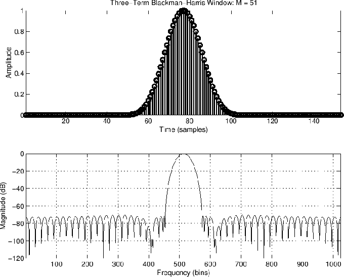
Figure 3.15: Longer three-term Blackman-Harris window and transform
FREQUENCY-DOMAIN IMPLEMENTATION OF THE
BLACKMAN-HARRIS FAMILY- Start with a length rectangular window
- Take an -point DFT
- Convolve the DFT data with the 3-point smoother

Note that the frequency-domain implementation of the Hann window requires no multiplies in linear fixed-point data formats [188].Similarly, any Blackman window may be implemented as a 5-point smoother in the frequency domain. More generally, any  -term Blackman-Harris window requires convolution of the critically sampled spectrum with a smoother of length -term Blackman-Harris window requires convolution of the critically sampled spectrum with a smoother of length  . .
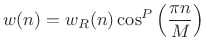
POWER-OF-COSINE WINDOW FAMILY
Definition:
where  is a nonnegative integer. is a nonnegative integer.
Properties: - The first terms of the window's Taylor expansion, evaluated at the endpoints are identically 0 .
- Roll-off rate
 dB/octave. dB/octave.
Special Cases:  Rectangular window Rectangular window MLT sine window MLT sine window Hann window (``raised cosine'' = `` '') Hann window (``raised cosine'' = `` '') Alternative Blackman (maximized roll-off rate) Alternative Blackman (maximized roll-off rate)
Thus,  windows parametrize -term Blackman-Harris windows (for windows parametrize -term Blackman-Harris windows (for  ) which are configured to use all degrees-of-freedom to maximize roll-off rate. ) which are configured to use all degrees-of-freedom to maximize roll-off rate.
SPECTRUM ANALYSIS OF AN OBOE TONEIn this section we compare three FFT windows applied to an oboe recording. The examples demonstrate that more gracefully tapered windows support a larger spectral dynamic range, at the cost of reduced frequency resolution.
RECTANGULAR-WINDOWED OBOE RECORDINGFigure [url=https://www.dsprelated.com/freebooks/sasp/Spectrum_Analysis_Windows.html#figboeboxcar]3.16[/url]a shows a segment of two quasi periods from an oboe recording at the pitch C4, and Fig.[url=https://www.dsprelated.com/freebooks/sasp/Spectrum_Analysis_Windows.html#figboeboxcar]3.16[/url]b shows the corresponding FFT magnitude. The window length was set to the next integer greater than twice the period length in samples. The FFT size was set to the next power of 2 which was at least five times the window length (for a minimum zero-paddingfactor of 5). The complete Matlab script is listed in §[url=https://www.dsprelated.com/freebooks/sasp/Matlab_listing_oboeanal_m.html#secboeanal]F.2.5[/url].
Figure 3.16: (a) Rectangularly windowed segment of two periods from the steady state portion of an oboe recording of pitch `C4'. (b) Zero-padded FFT magnitude.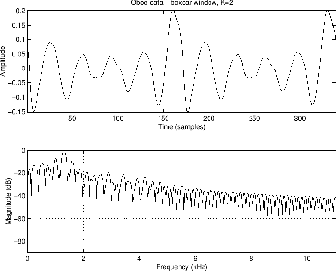
HAMMING-WINDOWED OBOE RECORDINGFigure [url=https://www.dsprelated.com/freebooks/sasp/Spectrum_Analysis_Windows.html#figboehamming]3.17[/url]a shows a segment of four quasi periods from the same oboe recording as in the previous figure multiplied by a Hamming window, and Fig.[url=https://www.dsprelated.com/freebooks/sasp/Spectrum_Analysis_Windows.html#figboehamming]3.17[/url]b shows the corresponding zero-padded FFT magnitude. Note how the lower side-lobes of the Hamming window significantly improve the visibility of spectral components above 6 kHz or so.
Figure 3.17: (a) Hamming-windowed segment of four periods from the steady state portion of an oboe recording of pitch `C4'. (b) Zero-padded FFT magnitude.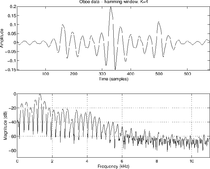
BLACKMAN-WINDOWED OBOE RECORDINGFigure [url=https://www.dsprelated.com/freebooks/sasp/Spectrum_Analysis_Windows.html#figboeblackman]3.18[/url]a shows a segment of six quasi periods from the same oboe recording as in Fig.[url=https://www.dsprelated.com/freebooks/sasp/Rectangular_Windowed_Oboe_Recording.html#figboeboxcar]3.16[/url] multiplied by a Blackman window, and Fig.[url=https://www.dsprelated.com/freebooks/sasp/Spectrum_Analysis_Windows.html#figboeblackman]3.18[/url]b shows the corresponding zero-padded FFT magnitude data. The lower side lobes of the Blackman window significantly improve over the Hamming-window results at high frequencies.
Figure 3.18: (a) Blackman-windowed segment of six periods from the steady state portion of an oboe recording of pitch `C4'. (b) Zero-padded FFT magnitude.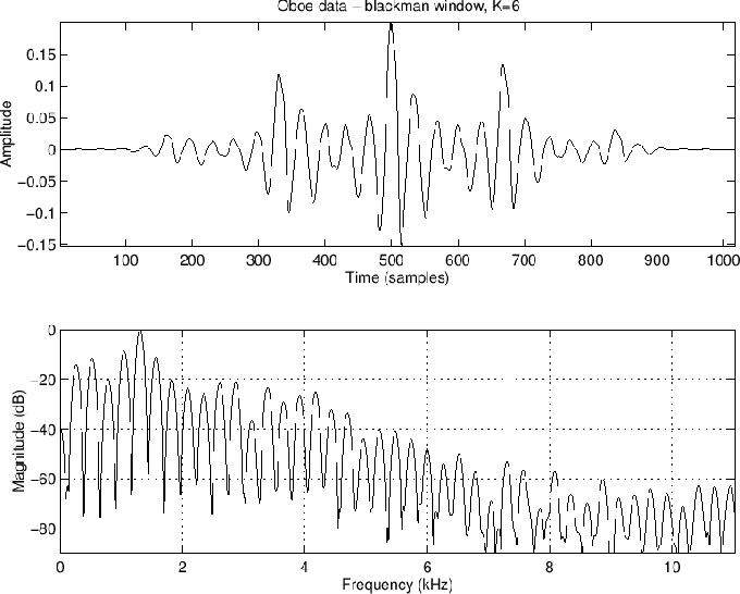
CONCLUSIONSNote that preemphasis (flattening the spectral envelope using a preemphasis filter) would have helped here by reducing the spectral dynamic range of the signal (see §10.3 for a number of methods). In voice signal processing, approximately  dB/octave preemphasis is common because voice spectra generally roll off at dB per octave [162]. If dB/octave preemphasis is common because voice spectra generally roll off at dB per octave [162]. If  denotes the original voice spectrum and denotes the original voice spectrum and  the preemphasized spectrum, then one method is to use a ``leaky first-order difference'' the preemphasized spectrum, then one method is to use a ``leaky first-order difference''
For voice signals, the preemphasized spectrum  tends to have a relatively ``flat'' magnitude envelope compared to tends to have a relatively ``flat'' magnitude envelope compared to  . This preemphasis can be taken out (inverted) by the simple one-pole filter . This preemphasis can be taken out (inverted) by the simple one-pole filter  . .
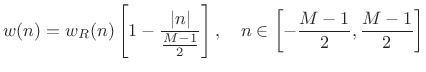
BARTLETT (``TRIANGULAR'') WINDOWThe Bartlett window (or simply triangular window) may be defined by
and the corresponding transform is
The following properties are immediate: - Convolution of two length
 rectangular windows rectangular windows - Main lobe twice as wide as that of a rectangular window of length
- First side lobe twice as far down as rectangular case (-26 dB)
- Often applied implicitly to sample correlations of finite data
- Also called the ``tent function''
- Can replace by
 to avoid including endpoint zeros to avoid including endpoint zeros
MATLAB FOR THE BARTLETT WINDOW:w = bartlett(M);This is equivalent, for odd , tow = 2*(0 M-1)/2)/(M-1);w = [w w((M-1)/2:-1:1)]';Note that, in contrast to the hanning function, but like the hann function, bartlett explicitly includes zeros at its endpoints:>> bartlett(3)ans = 0 1 0The triang function in Matlab implements the triangular window corresponding to the hanningcase:>> triang(3)ans = 0.5000 1.0000 0.5000 M-1)/2)/(M-1);w = [w w((M-1)/2:-1:1)]';Note that, in contrast to the hanning function, but like the hann function, bartlett explicitly includes zeros at its endpoints:>> bartlett(3)ans = 0 1 0The triang function in Matlab implements the triangular window corresponding to the hanningcase:>> triang(3)ans = 0.5000 1.0000 0.5000
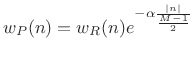
POISSON WINDOWThe Poisson window (or more generically exponential window) can be written
where determines the time constant :
where denotes the sampling interval in seconds.
Figure 3.19: The Poisson (exponential) window.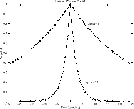
The Poisson window is plotted in Fig.3.19. In the  plane, the Poisson window has the effect of radially contracting the unit circle. Consider an infinitely long Poisson window (no truncation by a rectangular window plane, the Poisson window has the effect of radially contracting the unit circle. Consider an infinitely long Poisson window (no truncation by a rectangular window  ) applied to a causal signal ) applied to a causal signal  having transform having transform  : :
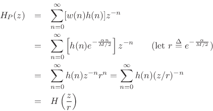
Thus, the unit-circle response is moved to  . This means, for example, that marginally stable poles in now decay as . This means, for example, that marginally stable poles in now decay as  in in  . . The effect of this radial -plane contraction is shown in Fig.3.20.
Figure 3.20: Radial contraction of the unit circle in the plane by the Poisson window.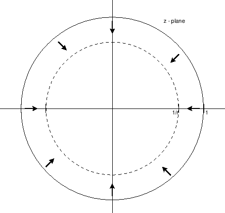
The Poisson window can be useful for impulse-response modeling by poles and/or zeros (``system identification''). In such applications, the window length is best chosen to include substantially all of the impulse-response data.
HANN-POISSON WINDOW
Definition:
Figure 3.21: Hann-Poisson window (upper plot, circles) and Fourier transform (lower plot). The upper plot also shows (using solid lines) the Hann and Poisson windows that are multiplied pointwise to produce the Hann-Poisson window.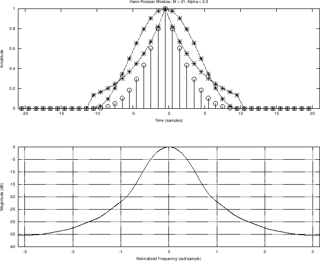
The Hann-Poisson window is, naturally enough, a Hann window times a Poisson window (exponential times raised cosine). It is plotted along with its DTFT in Fig.3.21. The Hann-Poisson window has the very unusual feature among windows of having ``no side lobes'' in the sense that, for  , the window-transform magnitude has negative slope for all positive frequencies [58], as shown in Fig.3.22. As a result, this window is valuable for ``hill climbing'' optimization methods such as Newton's method or any convex optimizationmethods. In other terms, of all windows we have seen so far, only the Hann-Poisson window has a convex transform magnitude to the left or right of the peak (Fig.3.21b). , the window-transform magnitude has negative slope for all positive frequencies [58], as shown in Fig.3.22. As a result, this window is valuable for ``hill climbing'' optimization methods such as Newton's method or any convex optimizationmethods. In other terms, of all windows we have seen so far, only the Hann-Poisson window has a convex transform magnitude to the left or right of the peak (Fig.3.21b).
Figure 3.22: Hann-Poisson Slope and Curvature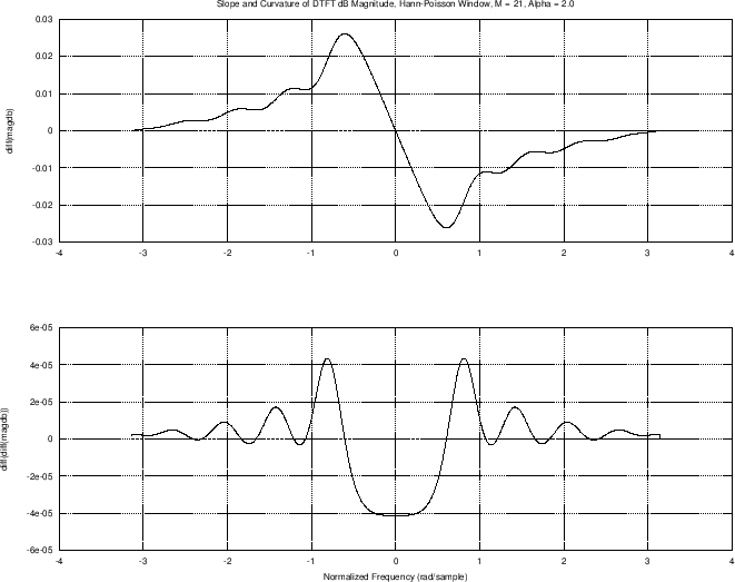
Figure 3.23 also shows the slope and curvature of the Hann-Poisson window transform, but this time with increased to 3. We see that higher further smooths the side lobes, and even the curvature becomes uniformly positive over a broad center range.
Figure 3.23: Hann-Poisson magnitude, slope, and curvature, in the frequency domain, for larger .
MATLAB FOR THE HANN-POISSON WINDOW
function [w,h,p] = hannpoisson(M,alpha)%HANNPOISSON - Length M Hann-Poisson windowMo2 = (M-1)/2; n=(-Mo2:Mo2)';scl = alpha / Mo2;p = exp(-scl*abs(n));scl2 = pi / Mo2;h = 0.5*(1+cos(scl2*n));w = p.*h;
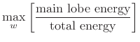
SLEPIAN OR DPSS WINDOWA window having maximal energy concentration in the main lobe is given by the digital prolate spheroidal sequence (DPSS) of order 0 [256,136]. It is obtained by using all degrees of freedom (sample values) in an -point window  to obtain a window transform to obtain a window transform  which maximizes the energy in the main lobe of the window relative to total energy: which maximizes the energy in the main lobe of the window relative to total energy:
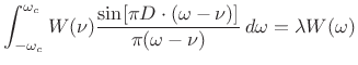
In the continuous-time case, i.e., when  is a continuous function of is a continuous function of  , the function which maximize this ratio is the first prolate spheroidal wave function for the given main-lobe bandwidth , the function which maximize this ratio is the first prolate spheroidal wave function for the given main-lobe bandwidth  [101], [202, p. 205].4.8 [101], [202, p. 205].4.8A prolate spheroidal wave function is defined as an eigenfunction of the integral equation
where  is the nonzero duration of is the nonzero duration of  in seconds. This integral equation can be understood as ``cropping'' to zero outside its main lobe (note that the integral goes from in seconds. This integral equation can be understood as ``cropping'' to zero outside its main lobe (note that the integral goes from  to to  , followed by a convolution of with a sinc function which ``time limits'' the window to a duration of seconds centered at time 0 in the time domain. In operator notation, , followed by a convolution of with a sinc function which ``time limits'' the window to a duration of seconds centered at time 0 in the time domain. In operator notation,
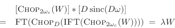
where  is a rectangular windowing operation which zeros outside the interval is a rectangular windowing operation which zeros outside the interval  . . Satisfying (3.37) means that window transform is an eigenfunction of this sequence of operations; that is, it can be zeroed outside the interval  , inverse Fourier transformed, zeroed outside the interval , inverse Fourier transformed, zeroed outside the interval  , and forward Fourier transformed to yield the original Window transform multiplied by some scale factor , and forward Fourier transformed to yield the original Window transform multiplied by some scale factor  (the eigenvalueof the overall operation). We may say that (the eigenvalueof the overall operation). We may say that  is the bandlimited extrapolation of its main lobe. is the bandlimited extrapolation of its main lobe. The sinc function in (3.37) can be regarded as a symmetric Toeplitz operator kernel), and the integral of multiplied by this kernel can be called a symmetric Toeplitz operator. This is a special case of a Hermitian operator, and by the general theory of Hermitian operators, there exists an infinite set of mutually orthogonal functions  , each associated with a real eigenvalues , each associated with a real eigenvalues  .4.9 If .4.9 If  denotes the largest such eigenvalue of (3.37), then its corresponding eigenfunction, denotes the largest such eigenvalue of (3.37), then its corresponding eigenfunction,  , is what we want as our Slepian window, orprolate spheroidal window in the continuous-time case. It is optimal in the sense of having maximum main-lobe energy as a fraction of total energy. , is what we want as our Slepian window, orprolate spheroidal window in the continuous-time case. It is optimal in the sense of having maximum main-lobe energy as a fraction of total energy. The discrete-time counterpart is Digital Prolate Spheroidal Sequences (DPSS), which may be defined as the eigenvectors of the following symmetric Toeplitz matrix constructed from a sampled sinc function [13]:
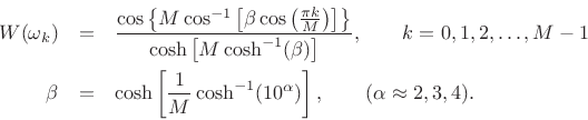
where denotes the desired window length in samples, is the desired main-lobe cut-off frequency in radians per second, and is the sampling period in seconds. The main-lobe bandwidth is thus rad/sec, counting both positive and negative frequencies.) The digital Slepian window (or DPSS window) is then given by the eigenvector corresponding to the largest eigenvalue. A simple matlab program is given in §F.1.2 for computing these windows, and facilities in Matlab and Octave are summarized in the next subsection.
MATLAB FOR THE DPSS WINDOWThe function dpss in the Matlab Signal Processing Tool Box4.10 can be used to compute them as follows: w = dpss(M,alpha,1); % discrete prolate spheroidal sequencewhere is the desired window length, and  can be interpreted as half of the window's time-bandwidth product can be interpreted as half of the window's time-bandwidth product  in ``cycles''. Alternatively, can be interpreted as the highest bin number in ``cycles''. Alternatively, can be interpreted as the highest bin number  inside the main lobe of the window transform inside the main lobe of the window transform 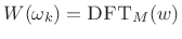 , when the DFT length is equal to the window length . (See the next section on the Kaiser window for more on this point.) , when the DFT length is equal to the window length . (See the next section on the Kaiser window for more on this point.)Some examples of DPSS windows and window transforms are given in Fig.3.29.
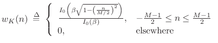
KAISER WINDOWJim Kaiser discovered a simple approximation to the DPSS window based upon Bessel functions [115], generally known as the Kaiser window (or Kaiser-Bessel window).
Definition:
Window transform: The Fourier transform of the Kaiser window  (where (where  is treated as continuous) is given by4.11 is treated as continuous) is given by4.11
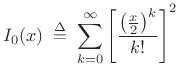
where  is the zero-order modified Bessel function of the first kind:4.12 is the zero-order modified Bessel function of the first kind:4.12
Notes:- Reduces to rectangular window for
 - Asymptotic roll-off is 6 dB/octave
- First null in window transform is at
 - Time-bandwidth product
 radians if bandwidths are measured from 0 to positive band-limit radians if bandwidths are measured from 0 to positive band-limit - Full time-bandwidth product
 radians when frequency bandwidth is defined as main-lobe width out to first null radians when frequency bandwidth is defined as main-lobe width out to first null - Sometimes the Kaiser window is parametrized by , where
KAISER WINDOW BETA PARAMETERThe parameter of the Kaiser window provides a convenient continuous control over the fundamental window trade-off between side-lobe level and main-lobe width. Larger values give lower side-lobe levels, but at the price of a wider main lobe. As discussed in §5.4.1, widening the main lobe reduces frequency resolution when the window is used for spectrum analysis. As explored in Chapter 9, reducing the side lobes reduces ``channel cross talk'' in an FFT-based filter-bank implementation. The Kaiser beta parameter can be interpreted as 1/4 of the ``time-bandwidth product''  of the window in radians (seconds times radians-per-second).4.13 Sometimes the Kaiser window is parametrized by of the window in radians (seconds times radians-per-second).4.13 Sometimes the Kaiser window is parametrized by  instead of . The parameter is therefore half the window's time-bandwidth product in cycles (seconds times cycles-per-second). instead of . The parameter is therefore half the window's time-bandwidth product in cycles (seconds times cycles-per-second).
KAISER WINDOWS AND TRANSFORMSFigure 3.24 plots the Kaiser window and its transform for 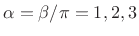 . Note how increasing causes the side-lobes to fall away from the main lobe. The curvature at the main lobe peak also decreases somewhat. . Note how increasing causes the side-lobes to fall away from the main lobe. The curvature at the main lobe peak also decreases somewhat.
Figure 3.24: Kaiser window and transform for  . .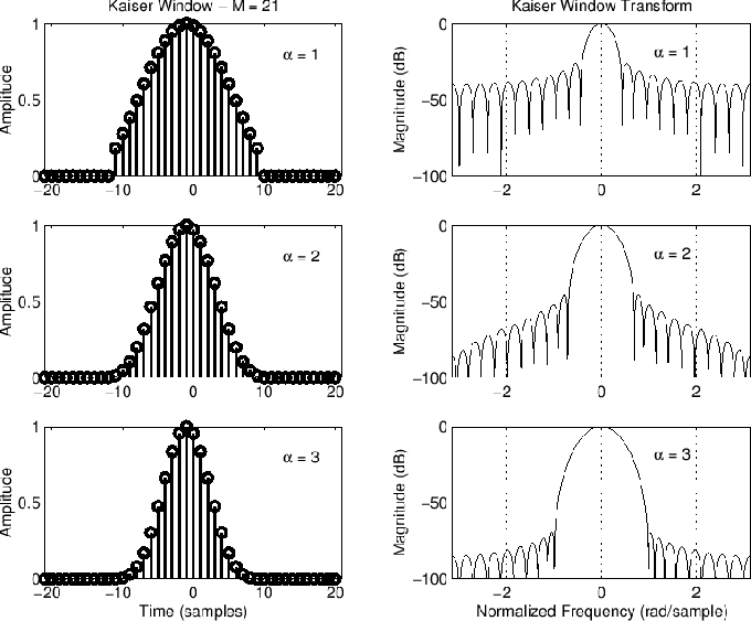
Figure 3.25 shows a plot of the Kaiser window for various values of  . Note that for , the Kaiser window reduces to the rectangular window. . Note that for , the Kaiser window reduces to the rectangular window.
Figure 3.25: The Kaiser window for various values of the time-bandwidth parameter .
Figure 3.26 shows a plot of the Kaiser window transforms for 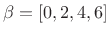 . For (top plot), we see the dB magnitude of the aliased sinc function. As increases the main-lobe widens and the side lobes go lower, reaching almost 50 dB down for . For (top plot), we see the dB magnitude of the aliased sinc function. As increases the main-lobe widens and the side lobes go lower, reaching almost 50 dB down for  . .
Figure 3.26: Kaiser window transform magnitude for various .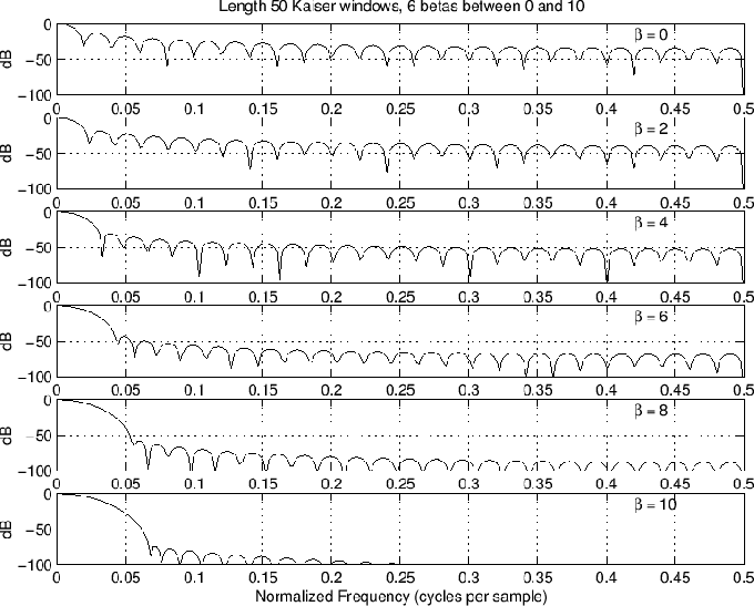
Figure 3.27 shows the effect of increasing window length for the Kaiser window. The window lengths are  from the top to the bottom plot. As with all windows, increasing the length decreases the main-lobe width, while the side-lobe level remains essentially unchanged. from the top to the bottom plot. As with all windows, increasing the length decreases the main-lobe width, while the side-lobe level remains essentially unchanged.
Figure 3.27: Kaiser window transform magnitudes for various window lengths.
Figure 3.28 shows a plot of the Kaiser window side-lobe level for various values of 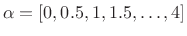 . For , the Kaiser window reduces to the rectangular window, and we expect the side-lobe level to be about 13 dB below the main lobe (upper-lefthand corner of Fig.3.28). As . For , the Kaiser window reduces to the rectangular window, and we expect the side-lobe level to be about 13 dB below the main lobe (upper-lefthand corner of Fig.3.28). As  increases, the dB side-lobe level reduces approximately linearly with main-lobe width increase (approximately a 25 dB drop in side-lobe level for each main-lobe width increase by one sinc-main-lobe). increases, the dB side-lobe level reduces approximately linearly with main-lobe width increase (approximately a 25 dB drop in side-lobe level for each main-lobe width increase by one sinc-main-lobe).
Figure 3.28: Kaiser window side-lobe level for various values of .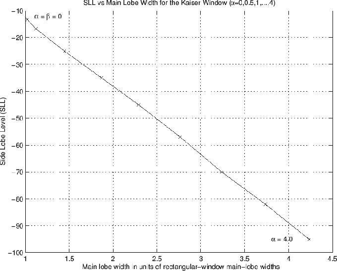
MINIMUM FREQUENCY SEPARATION VS. WINDOW LENGTHThe requirements on window length for resolving closely tuned sinusoids was discussed in §5.5.2. This section considers this issue for the Kaiser window. Table 3.1 lists the parameter required for a Kaiser window to resolve equal-amplitude sinusoids with a frequency spacing of  rad/sample [1, Table 8-9]. Recall from §3.9 that can be interpreted as half of the time-bandwidth of the window (in cycles). rad/sample [1, Table 8-9]. Recall from §3.9 that can be interpreted as half of the time-bandwidth of the window (in cycles).
Table:Kaiser parameter for various frequency resolutions, assuming an FFTzero-paddingfactor of at least 3.5.
1.5
2.0
2.5
3.0
KAISER AND DPSS WINDOWS COMPAREDFigure 3.29 shows an overlay of DPSS and Kaiser windows for some different values. In all cases, the window length was  . Note how the two windows become more similar as increases. The Matlab for computing the windows is as follows: . Note how the two windows become more similar as increases. The Matlab for computing the windows is as follows: w1 = dpss(M,alpha,1); % discrete prolate spheroidal seq. w2 = kaiser(M,alpha*pi); % corresponding kaiser window
Figure: Comparison of length 51 DPSS and Kaiser windows for  . .
The following Matlab comparison of the DPSS and Kaiser windows illustrates the interpretation of as the bin number of the edge of the critically sampled window main lobe, i.e., when the DFT length equals the window length: format long;M=17;alpha=5;abs(fft([ dpss(M,alpha,1), kaiser(M,pi*alpha)/2]))ans = 2.82707022360190 2.50908747431366 2.00652719015325 1.92930705688346 0.68469697658600 0.85272343521683 0.09415916813555 0.19546670371747 0.00311639169878 0.01773139505899 0.00000050775691 0.00022611995322 0.00000003737279 0.00000123787805 0.00000000262633 0.00000066206722 0.00000007448708 0.00000034793207 0.00000007448708 0.00000034793207 0.00000000262633 0.00000066206722 0.00000003737279 0.00000123787805 0.00000050775691 0.00022611995322 0.00311639169878 0.01773139505899 0.09415916813555 0.19546670371747 0.68469697658600 0.85272343521683 2.00652719015325 1.92930705688346Finally, Fig.3.30 shows a comparison of DPSS and Kaiser window transforms, where the DPSS window was computed using the simple method listed in §F.1.2. We see that the DPSS window has a slightly narrower main lobe and lower overall side-lobe levels, although its side lobes are higher far from the main lobe. Thus, the DPSS window has slightly better overall specifications, while Kaiser-window side lobes have a steeper roll off.
Figure: DPSS and Kaiser window transforms, for length  , DPSS cut-off , DPSS cut-off  , and Kaiser , and Kaiser  . .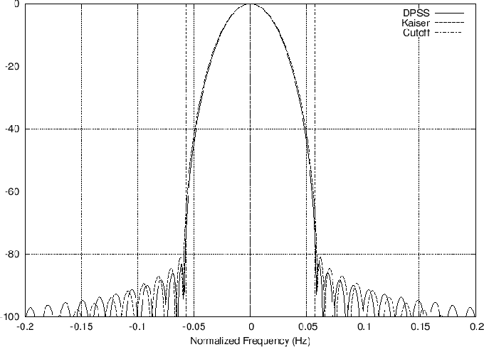
DOLPH-CHEBYSHEV WINDOW
 \omega_c} \left\vert W(\omega)\right\vert\right\}$" style="border: 0px;"> | (4.43) |
The Chebyshev norm is also called the  norm, uniform norm, minimax norm, or simply the maximum absolute value. norm, uniform norm, minimax norm, or simply the maximum absolute value.An equivalent formulation is to minimize main-lobe width subject to a side-lobe specification:
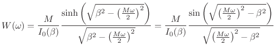
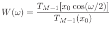
The optimal Dolph-Chebyshev window transform can be written in closed form [61,101,105,156]:
The zero-phase Dolph-Chebyshev window, , is then computed as the inverse DFT of  .4.14 The parameter controls the side-lobe level via the formula [156] .4.14 The parameter controls the side-lobe level via the formula [156]
Side-Lobe Level in dB | (4.45) |
Thus,  gives side-lobes which are gives side-lobes which are  dB below the main-lobe peak. Since the side lobes of the Dolph-Chebyshev window transform are equal height, they are often called ``ripple in the stop-band'' (thinking now of the window transform as a lowpass filter frequency response). The smaller the ripple specification, the larger has to become to satisfy it, for a given window length . dB below the main-lobe peak. Since the side lobes of the Dolph-Chebyshev window transform are equal height, they are often called ``ripple in the stop-band'' (thinking now of the window transform as a lowpass filter frequency response). The smaller the ripple specification, the larger has to become to satisfy it, for a given window length .
MATLAB FOR THE DOLPH-CHEBYSHEV WINDOWw = chebwin(31,60);designs a length  window with side lobes at window with side lobes at  dB (when the main-lobe peak is normalized to 0 dB). dB (when the main-lobe peak is normalized to 0 dB).
EXAMPLE CHEBYSHEV WINDOWS AND TRANSFORMSFigure 3.31 shows the Dolph-Chebyshev window and its transform as designed by chebwin(31,40) in Matlab, and Fig.3.32 shows the same thing for chebwin(31,200). As can be seen from these examples, higher side-lobe levels are associated with a narrower main lobe and more discontinuous endpoints.
Figure: The length  Dolph-Chebyshev window with ripple (side-lobe level) specified to be Dolph-Chebyshev window with ripple (side-lobe level) specified to be  dB. dB.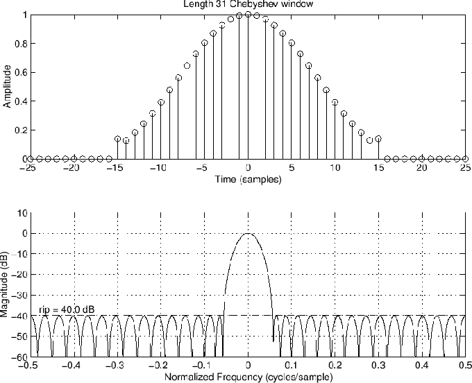
Figure: The length Dolph-Chebyshev window with ripple (side-lobe level) specified to be  dB. dB.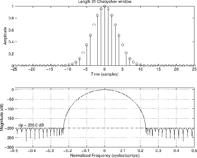
Figure: The length  Dolph-Chebyshev window with ripple (side-lobe level) specified to be dB. Dolph-Chebyshev window with ripple (side-lobe level) specified to be dB.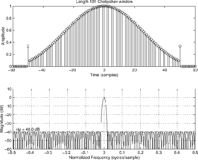
Figure 3.33 shows the Dolph-Chebyshev window and its transform as designed by chebwin(101,40) in Matlab. Note how the endpoints have actually become impulsive for the longer window length. The Hamming window, in contrast, is constrained to be monotonic away from its center in the time domain. The ``equal ripple'' property in the frequency domain perfectly satisfies worst-case side-lobe specifications. However, it has the potentially unfortunate consequence of introducing ``impulses'' at the window endpoints. Such impulses can be the source of ``pre-echo'' or ``post-echo'' distortion which are time-domain effects not reflected in a simple side-lobe level specification. This is a good lesson in the importance of choosing the right error criterion to minimize. In this case, to avoid impulse endpoints, we might add a continuity or monotonicity constraint in the time domain (see §3.13.2 for examples).
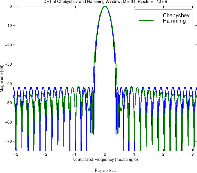
CHEBYSHEV AND HAMMING WINDOWS COMPAREDFigure 3.34 shows an overlay of Hamming and Dolph-Chebyshev window transforms, the ripple parameter for chebwin set to  dB to make it comparable to the Hamming side-lobelevel. We see that the monotonicity constraint inherent in the Hamming window family only costs a few dB of deviation from optimality in the Chebyshev sense at high frequency. dB to make it comparable to the Hamming side-lobelevel. We see that the monotonicity constraint inherent in the Hamming window family only costs a few dB of deviation from optimality in the Chebyshev sense at high frequency.
DOLPH-CHEBYSHEV WINDOW THEORYIn this section, the main elements of the theory behind the Dolph-Chebyshev window are summarized.
CHEBYSHEV POLYNOMIALS
Figure 3.34: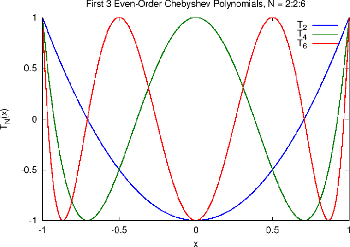
The  th Chebyshev polynomial may be defined by th Chebyshev polynomial may be defined by
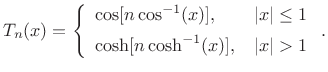 1 \\ \end{array} \right..$" style="border: 0px;"> | (4.46) |
The first three even-order cases are plotted in Fig.3.35. (We will only need the even orders for making Chebyshev windows, as only they are symmetric about time 0.) Clearly,  and and  . Using the double-angle trig formula . Using the double-angle trig formula  , it can be verified that , it can be verified that
for  . The following properties of the Chebyshev polynomials are well known: . The following properties of the Chebyshev polynomials are well known: is an th-order polynomial in is an th-order polynomial in  . .- is an even function when is an even integer, and odd when is odd.
- has zeros in the open interval
 , and , and  extrema in the closed interval extrema in the closed interval  . .  1$" style="border: 0px;"> for 1$" style="border: 0px;"> for  1$" style="border: 0px;"> . 1$" style="border: 0px;"> .
DOLPH-CHEBYSHEV WINDOW DEFINITION
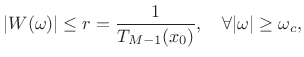
where  1$" style="border: 0px;"> is defined by the desired ripple specification: 1$" style="border: 0px;"> is defined by the desired ripple specification:
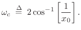
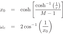
where is the ``main lobe edge frequency'' defined by
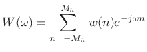
Expanding in terms of complex exponentials yields
where  . Thus, the coefficients give the length Dolph-Chebyshev window in zero-phase form. . Thus, the coefficients give the length Dolph-Chebyshev window in zero-phase form.
DOLPH-CHEBYSHEV WINDOW MAIN-LOBE WIDTHGiven the window length and ripple magnitude  , the main-lobe width may be computed as follows [155]: , the main-lobe width may be computed as follows [155]:
This is the smallest main-lobe width possible for the given window length and side-lobe spec.
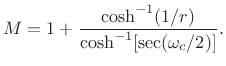
DOLPH-CHEBYSHEV WINDOW LENGTH COMPUTATIONGiven a prescribed side-lobe ripple-magnitude and main-lobe width , the required window length is given by [155]
For  (the typical case), the denominator is close to (the typical case), the denominator is close to  , and we have , and we have
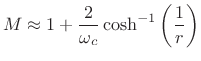
Thus, half the time-bandwidth product in radians is approximately
where is the parameter often used to design Kaiser windows (§3.9).
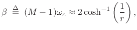
GAUSSIAN WINDOW AND TRANSFORMThe Gaussian ``bell curve'' is possibly the only smooth, nonzero function, known in closed form, that transforms to itself.4.15
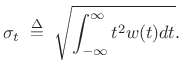
It also achieves the minimum time-bandwidth product
when ``width'' is defined as the square root of its second central moment. For even functions ,
Since the true Gaussian function has infinite duration, in practice we must window it with some usual finite window, or truncate it. Depalle [58] suggests using a triangular window raised to some power for this purpose, which preserves the absence of side lobes for sufficiently large . It also preserves non-negativity of the transform.
MATLAB FOR THE GAUSSIAN WINDOWIn matlab, w = gausswin(M,alpha) returns a length window with parameter 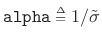 where where  is defined, as in Harris [101], so that the window shape is invariant with respect to window length : is defined, as in Harris [101], so that the window shape is invariant with respect to window length : function [w] = gausswin(M,alpha)n = -(M-1)/2 : (M-1)/2;w = exp((-1/2) * (alpha * n/((M-1)/2)) .^ 2)';An implementation in terms of unnormalized standard deviation (sigma in samples) is as follows: function [w] = gaussianwin(M,sigma)n= -(M-1)/2 : (M-1)/2;w = exp(-n .* n / (2 * sigma * sigma))';In this case, sigma would normally be specified as a fraction of the window length (sigma = M/8 in the sample below).Note that, on a dB scale, Gaussians are quadratic. This means that parabolic interpolation of a sampled Gaussian transform is exact. This can be a useful fact to remember when estimating sinusoidal peak frequencies in spectra. For example, one suggested implication is that, for typical windows, quadratic interpolation of spectral peaks may be more accurate on a log-magnitude scale (e.g., dB) than on a linear magnitude scale (this has been observed empirically for a variety of cases).
GAUSSIAN WINDOW AND TRANSFORMFigure 3.36 shows an example length Gaussian window and its transform. The sigmaparameter was set to  so that simple truncation of the Gaussian yields a side-lobe level better than so that simple truncation of the Gaussian yields a side-lobe level better than  dB. Also overlaid on the window transform is a parabola; we see that the main lobe is well fit by the parabola until the side lobes begin. Since the transform of a Gaussian is a Gaussian (exactly), the side lobes are entirely caused by truncating the window. dB. Also overlaid on the window transform is a parabola; we see that the main lobe is well fit by the parabola until the side lobes begin. Since the transform of a Gaussian is a Gaussian (exactly), the side lobes are entirely caused by truncating the window.
Figure 3.36: Gaussian window and transform.
EXACT DISCRETE GAUSSIAN WINDOWIt can be shown [44] that
where  is the time index, and is the time index, and  is the frequency index for a length (even) normalized DFT (DFT divided by is the frequency index for a length (even) normalized DFT (DFT divided by  ). In other words, the Normalized DFT (NDFT) of this particular sampled Gaussian pulse is exactly the complex-conjugate of the same Gaussian pulse. (The proof is nontrivial.) ). In other words, the Normalized DFT (NDFT) of this particular sampled Gaussian pulse is exactly the complex-conjugate of the same Gaussian pulse. (The proof is nontrivial.)
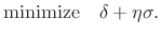
OPTIMIZED WINDOWSWe close this chapter with a general discussion of optimal windows in a wider sense. We generally desire
but the nature of this approximation is typically determined by characteristics of audio perception. Best results are usually obtained by formulating this as an FIR filter designproblem (see Chapter 4). In general, both time-domain and frequency-domain specifications are needed. (Recall the potentially problematic impulses in the Dolph-Chebyshev windowshown in Fig.3.33 when its length was long and ripple level was high). Equivalently, both magnitude and phase specifications are necessary in the frequency domain.A window transform can generally be regarded as the frequency response of a lowpass filterhaving a stop band corresponding to the side lobes and a pass band corresponding to the main lobe (or central section of the main lobe). Optimal lowpass filters require a transition region from the pass band to the stop band. For spectrum analysis windows, it is natural to define the entire main lobe as ``transition region.'' That is, the pass-band width is zero. Alternatively, the pass-band could be allowed to have a finite width, allowing some amount of ``ripple'' in the pass band; in this case, the pass-band ripple will normally be maximum at the main-lobe midpoint (  , say), and at the pass-band edges ( , say), and at the pass-band edges (  ). By embedding the window design problem within the more general problem of FIR digital filter design, a plethora of optimal design techniques can be brought to bear [204,258,14,176,218]. ). By embedding the window design problem within the more general problem of FIR digital filter design, a plethora of optimal design techniques can be brought to bear [204,258,14,176,218].
OPTIMAL WINDOWS FOR AUDIO CODINGRecently, numerically optimized windows have been developed by Dolby which achieve the following objectives: - Narrow the window in time
- Smooth the onset and decay in time
- Reduce side lobes below the worst-case masking threshold
See [200] for an overview. This is an excellent example of how window design should be driven by what one really wants.See §[url=https://www.dsprelated.com/freebooks/sasp/Optimal_FIR_Digital_Filter.html#secptimalfir]4.10[/url] for an overview of optimal methods for FIR digital filter design.
GENERAL RULEThere is rarely a closed form expression for the optimal window in practice. The most important task is to formulate an ideal error criterion. Given the right error criterion, it is usually straightforward to minimize it numerically with respect to the window samples  . .
WINDOW DESIGN BY LINEAR PROGRAMMINGThis section, based on a class project by EE graduate student Tatsuki Kashitani, illustrates the use of linprog in Matlab for designing variations on the Chebyshev window (§3.10). In addition, some comparisons between standard linear programming and the Remez exchange algorithm (firpm) are noted.
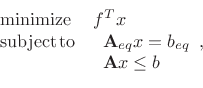
LINEAR PROGRAMMING (LP)If we can get our filter or window design problems in the form
where  , ,  , ,  is is  , etc., then we are done. , etc., then we are done.The linprog function in Matlab Optimization Toolbox solves LP problems. In Octave, one can use glpk instead (from the GNU GLPK library).
LP FORMULATION OF CHEBYSHEV WINDOW DESIGNWhat we want:
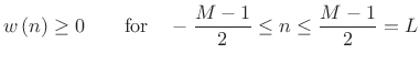
- Symmetric zero-phase window.
- Window samples to be positive.
- Transform to be 1 at DC.
- Transform to be within
 in the stop-band. in the stop-band.
- And
 to be small. to be small.
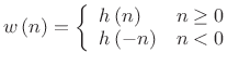
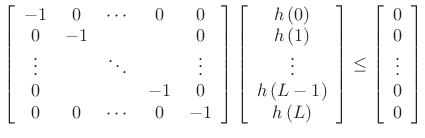
SYMMETRIC WINDOW CONSTRAINT
POSITIVE WINDOW-SAMPLE CONSTRAINTFor each window sample,  , or, , or,
Stacking inequalities for all ,
or
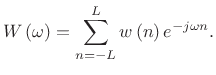
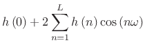
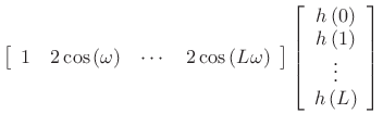
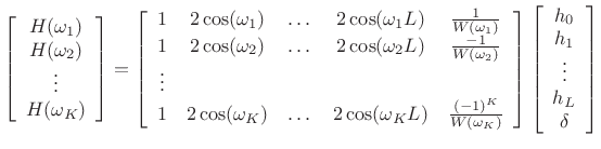
DC CONSTRAINTThe DTFT at frequency  is given by is given by
By zero-phase symmetry,
So  can be expressed as can be expressed as
 | (4.70) |
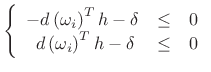
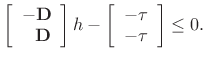
SIDELOBE SPECIFICATIONLikewise, side-lobe specification can be enforced at frequencies  in the stop-band. in the stop-band.
or
where
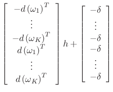
We need  to obtain many frequency samples per side lobe. Stacking inequalities for all , to obtain many frequency samples per side lobe. Stacking inequalities for all ,
I.e.,
 | (4.74) |
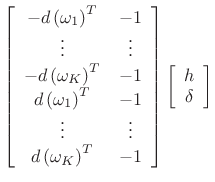
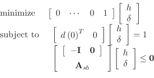
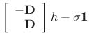
LP STANDARD FORMNow gather all of the constraints to form an LP problem:
where the optimization variables are  . .Solving this linear-programming problem should produce a window that is optimal in the Chebyshev sense over the chosen frequency samples, as shown in Fig.3.37. If the chosen frequency samples happen to include all of the extremal frequencies (frequencies of maximum error in the DTFT of the window), then the unique Chebyshev window for the specified main-lobe width must be obtained. Iterating to find the extremal frequencies is the heart of the Remez multiple exchange algorithm, discussed in the next section.
Figure 3.37: Normal Chebyshev Window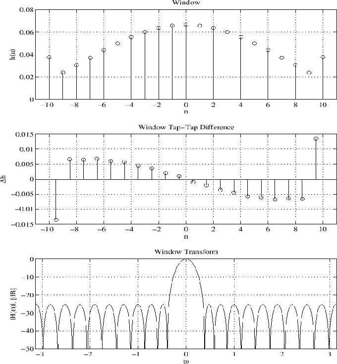
REMEZ EXCHANGE ALGORITHMThe Remez multiple exchange algorithm works by moving the frequency samples each iteration to points of maximum error (on a denser grid). Remez iterations could be added to our formulation as well. The Remez multiple exchange algorithm (function firpm [formerly remez] in the Matlab Signal Processing Toolbox, and still remez in Octave) is normally faster than a linear programming formulation, which can be regarded as a single exchange method [224, p. 140]. Another reason for the speed of firpm is that it solves the following equations non-iteratively for the filter exhibiting the desired error alternation over the current set of extremal frequencies:
where  is the weighted ripple amplitude at frequency is the weighted ripple amplitude at frequency  . ( is an arbitrary ripple weighting function.) Note that the desired frequency-response amplitude . ( is an arbitrary ripple weighting function.) Note that the desired frequency-response amplitude  is also arbitrary at each frequency sample. is also arbitrary at each frequency sample.
CONVERGENCE OF REMEZ EXCHANGEAccording to a theorem of Remez, is guaranteed to increase monotonically each iteration, ultimately converging to its optimal value. This value is reached when all the extremal frequencies are found. In practice, numerical round-off error may cause not to increase monotonically. When this is detected, the algorithm normally halts and reports a failure to converge. Convergence failure is common in practice for FIR filters having more than 300 or so taps and stringent design specifications (such as very narrow pass-bands). Further details on Remez exchange are given in [224, p. 136]. As a result of the non-iterative internal LP solution on each iteration, firpm cannot be used when additional constraints are added, such as those to be discussed in the following sections. In such cases, a more general LP solver such as linprog must be used. Recent advances in convex optimization enable faster solution of much larger problems [22].
MONOTONICITY CONSTRAINTWe can constrain the positive-time part of the window to be monotonically decreasing:
In matrix form,
or,
 | (4.78) |
See Fig.3.38.
Figure 3.38: Monotonic Chebyshev Window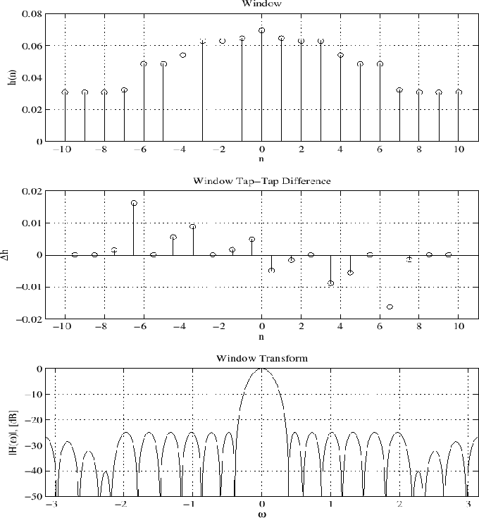
L-INFINITY NORM OF DERIVATIVE OBJECTIVEWe can add a smoothness objective by adding -norm of the derivative to the objective function.
The -norm only cares about the maximum derivative. Large  means we put more weight on the smoothness than the side-lobe level. means we put more weight on the smoothness than the side-lobe level. This can be formulated as an LP by adding one optimization parameter  which bounds all derivatives. which bounds all derivatives.
In matrix form,
Objective function becomes
 | (4.81) |
The result of adding the Chebyshev norm of diff(h) to the objective function to be minimized ( ) is shown in Fig.3.39. The result of increasing to 20 is shown in Fig.3.40. ) is shown in Fig.3.39. The result of increasing to 20 is shown in Fig.3.40.
Figure: Chebyshev norm of diff(h) added to the objective function to be minimized ( )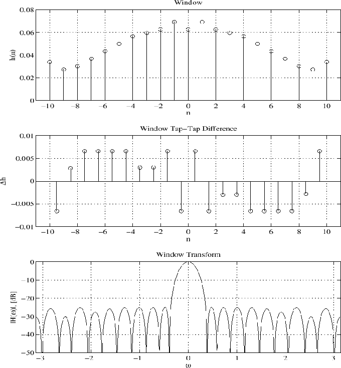
Figure: Twenty times the norm of diff(h) added to the objective function to be minimized ( ) )
L-ONE NORM OF DERIVATIVE OBJECTIVEAnother way to add smoothness constraint is to add  -norm of the derivative to the objective: -norm of the derivative to the objective:
Note that the norm is sensitive to all the derivatives, not just the largest.We can formulate an LP problem by adding a vector of optimization parameters which bound derivatives:
In matrix form,
The objective function becomes
See Fig.3.41 and Fig.3.42 for example results.
Figure: norm of diff(h) added to the objective function ( )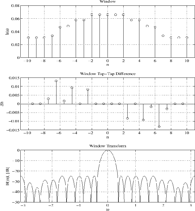
Figure: Six times the norm of diff(h) added to the objective function ( ) )
SUMMARYThis section illustrated the design of optimal spectrum-analysis windows made using linear-programming (linprog in matlab) or Remez multiple exchange algorithms (firpm in Matlab). After formulating the Chebyshev window as a linear programming problem, we found we could impose a monotonicity constraint on its shape in the time domain, or various derivative constraints. In Chapter 4, we will look at methods for FIR filter design, including the window method (§4.5) which designs FIR filters as a windowed ideal impulse response. The formulation introduced in this section can be used to design such windows, and it can be used to design optimal FIR filters. In such cases, the impulse response is designed directly (as the window was here) to minimize an error criterion subject to various equality and inequality constraints, as discussed above for window design.4.16
|


 发表于 2018-9-4 11:48:56


 min
min