https://www.dsprelated.com/freebooks/mdft/DB_Display.html
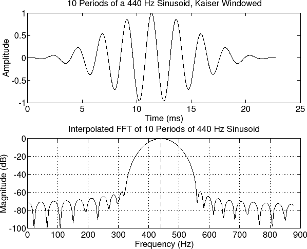
DB FOR DISPLAYIn practical signal processing, it is common to choose the maximum signal magnitude as the reference amplitude. That is, we normalize the signal so that the maximum amplitude is defined as 1, or 0 dB. This convention is also used by ``sound level meters'' in audio recording. When displaying magnitude spectra, the highest spectral peak is often normalized to 0 dB. We can then easily read off lower peaks as so many dB below the highest peak. Figure F.1b shows a plot of the Fast Fourier Transform (FFT) of ten periods of a ``Kaiser-windowed'' sinusoid at  Hz. (FFT windows are introduced in §8.1.4. The window is used to taper a finite-duration section of the signal.) Note that the peak dB magnitude has been normalized to zero, and that the plot has been clipped at -100 dB. Hz. (FFT windows are introduced in §8.1.4. The window is used to taper a finite-duration section of the signal.) Note that the peak dB magnitude has been normalized to zero, and that the plot has been clipped at -100 dB.
Figure F.1: Windowed sinusoid (top) and its FFT magnitude (bottom).
Below is the Matlab code for producing Fig.F.1. Note that it contains several elements (windows, zero padding, spectral interpolation) that we will not cover until later. They are included here as ``forward references'' in order to keep the example realistic and practical, and to give you an idea of ``how far we have to go'' before we know how to do practical spectrum analysis. Otherwise, the example just illustrates plotting spectra on an arbitrary dB scale between convenient limits. % Practical display of the fft of a synthesized sinusoidfs = 44100; % Sampling ratef = 440; % Sinusoidal frequency = A-440nper = 10; % Number of periods to synthesizedur = nper/f; % Duration in secondsT = 1/fs; % Sampling periodt = 0:T:dur; % Discrete-time axis in secondsL = length(t) % Number of samples to synthesizeZP = 5; % Zero padding factorN = 2^(nextpow2(L*ZP)) % FFT size (power of 2)x = cos(2*pi*f*t); % A sinusoid at A-440 ("row vector")w = kaiser(L,8); % An "FFT window"xw = x .* w'; % Need to transpose w to get a rowsound(xw,fs); % Might as well listen to itxzp = [xw,zeros(1,N-L)];% Zero-padded FFT input bufferX = fft(xzp); % Interpolated spectrum of xwXmag = abs(X); % Spectral magnitudeXdb = 20*log10(Xmag); % Spectral magnitude in dBXdbMax = max(Xdb); % Peak dB magnitudeXdbn = Xdb - XdbMax; % Normalize to 0dB peakdBmin = -100; % Don't show anything lower than thisXdbp = max(Xdbn,dBmin); % Normalized, clipped, dB mag specfmaxp = 2*f; % Upper frequency limit of plot, Hzkmaxp = fmaxp*N/fs; % Upper frequency limit of plot, binsfp = fs*[0:kmaxp]/N; % Frequency axis in Hz% Ok, plot it already!subplot(2,1,1);plot(1000*t,xw);xlabel('Time (ms)');ylabel('Amplitude');title(sprintf(['a) %d Periods of a %3.0f Hz Sinusoid, ', 'Kaiser Windowed'],nper,f)R);subplot(2,1,2);plot(fp,Xdbp(1:kmaxp+1)); grid;% Plot a dashed line where the peak should be: hold on; plot([440 440],[dBmin,0],'--'); hold off;xlabel('Frequency (Hz)');ylabel('Magnitude (dB)');title(sprintf(['b) Interpolated FFT of %d Periods of ',... '%3.0f Hz Sinusoid'],nper,f));The following more compact Matlab produces essentially the same plot, but without the nice physical units on the horizontal axes: x = cos([0:2*pi/20:10*2*pi]); % 10 periods, 20 samples/cycleL = length(x);xw = x' .* kaiser(L,8);N = 2^nextpow2(L*5);X = fft([xw',zeros(1,N-L)]);subplot(2,1,1); plot(xw);xlabel('Time (samples)'); ylabel('Amplitude');title('a) 10 Periods of a Kaiser-Windowed Sinusoid');subplot(2,1,2); kmaxp = 2*10*5; Xl = 20*log10(abs(X(1:kmaxp+1)));plot([10*5+1,10*5+1],[-100,0],[0:kmaxp],max(Xl-max(Xl),-100)); grid;xlabel('Frequency (Bins)'); ylabel('Magnitude (dB)');title('b) Interpolated FFT of 10 Periods of Sinusoid');
Next Section:
One's Complement Fixed-Point Format
Previous Section:
DBA (A-Weighted DB)
|